
Gradient Descent: Minimizing The Loss Function
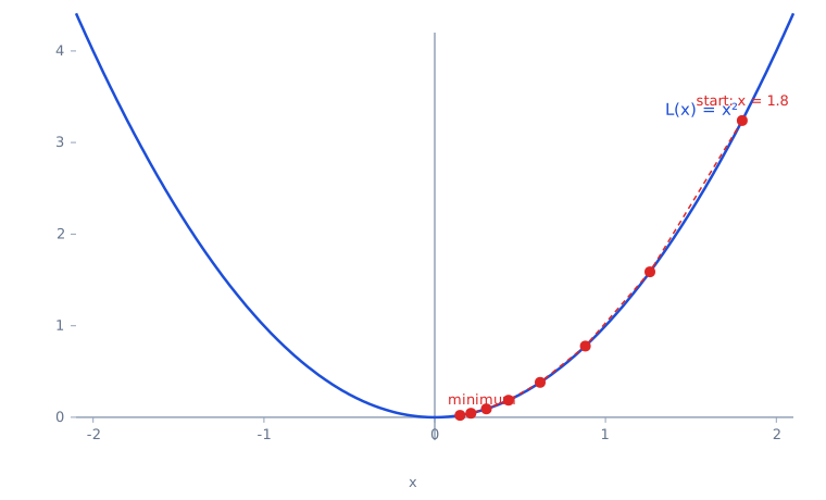
Visualizing Gradient Descent This plot shows gradient descent in action, where we try to minimize a simple loss function:
Backpropagation & Gradient Descent
Key Terms
- Gradient = Rate of Change = Derivative
- In deep learning, the gradient tells us how to adjust weights to reduce error
- Backpropagation computes gradients using the chain rule
- Gradient descent moves in the opposite direction of the gradient to improve predictions
Visualizing Gradient Descent
This plot shows gradient descent in action, where we try to minimize a simple loss function:
\(L(x) = x^2\)
What's Happening in the Graph?
- The blue curve represents the loss function, which is a simple U-shaped curve
- The goal is to reach the lowest point (where \(x = 0\))
- The red points show the path of gradient descent:
- We start at \(x = 1.8\) (far from the minimum)
- We compute the gradient (derivative) at that point
- We move in the opposite direction of the gradient to decrease the loss
- This process repeats until we reach the lowest point
- The red dashed line shows the step-by-step movement as we adjust \(x\) towards the minimum
How This Relates to Deep Learning
- In a neural network, each weight (parameter) has a gradient that tells us how to adjust it
- Backpropagation computes gradients for all weights using the chain rule
- Gradient descent updates the weights, just like in the example, moving towards the best solution
Putting it Together
- Gradient descent is just moving step by step downhill to minimize the loss
- The gradient (derivative) tells us which direction to move
- Backpropagation computes these gradients for every weight in the neural network
- By following the gradient, the model "learns" better predictions
Step-by-Step Walkthrough of Backpropagation and Gradients
Let's break it down into simple, clear steps so you understand exactly what's happening in the training process.
Step 1: Define the Simple Neural Network
class SimpleNN(torch.nn.Module):
    def __init__(self):
        super(SimpleNN, self).__init__()
        self.weight = torch.nn.Parameter(torch.tensor([2.0], requires_grad=True))  # Start with weight = 2

    def forward(self, x):
        return self.weight * x  # Simple linear model: y = weight * x
- 🔹 We create a simple neural network with one weight
- 🔹 The goal is for the weight to learn the correct value (which should be 4)
- 🔹
requires_grad=Truetells PyTorch to track gradients so we can apply backpropagation
Step 2: Define the Loss Function
loss_fn = torch.nn.MSELoss() # Mean Squared Error loss function
- 🔹 We use Mean Squared Error (MSE), which measures how far off our predictions are
- 🔹 Formula for MSE:
\(L = \frac{1}{n} \sum (y_{true} - y_{pred})^2\)
- If our model predicts badly, the loss is high
- If our model predicts well, the loss is low
Step 3: Define the Training Data
x_train = torch.tensor([1.0])  # Input value
y_train = torch.tensor([4.0])  # Expected output (goal is for weight to be 4)
- 🔹 We input \(x = 1\) into the model
- 🔹 We want the model to output \(y = 4\)
- 🔹 The model will adjust the weight until it learns to predict 4
Step 4: Forward Pass (Prediction)
y_pred = model(x_train) # Forward pass
- 🔹 The model makes a prediction using:
\(y_{pred} = weight \times x\)
- Initially, weight = 2, so:
\(y_{pred} = 2 \times 1 = 2\)
- But the correct answer is 4, so the model is wrong
Step 5: Compute the Loss
loss = loss_fn(y_pred, y_train) # Compute loss
- 🔹 We compute the MSE loss:
\(L = (4 - 2)^2 = 4\)
- The loss is high because the prediction is far from 4
- We need to reduce the loss by updating the weight
Step 6: Compute the Gradient (Backpropagation)
loss.backward() # Compute gradients
- 🔹 PyTorch automatically calculates the derivative of the loss function with respect to the weight
How does this work?
- Loss Function: \(L = (y_{\text{true}} - y_{\text{pred}})^2\)
- Since \(y_{\text{pred}} = \text{weight} \times x\), we take the derivative:
\(\frac{dL}{dweight} = 2 \times (y_{pred} - y_{true}) \times x\)
- Substituting \(y_{\text{pred}} = 2\) and \(y_{\text{true}} = 4\):
\(\frac{dL}{dweight} = 2 \times (2 - 4) \times 1 = -4\)
- This gradient tells us that if we increase the weight, the loss will decrease
Step 7: Update the Weight (Gradient Descent)
- 🔹 Gradient Descent Formula:
\(new\_weight = old\_weight - learning\_rate \times gradient\)
- Initially, weight = 2
- The computed gradient is -4
- We update the weight using learning rate = 0.1:
\(new\_weight = 2 - (0.1 \times (-4))\)
\(new\_weight = 2 + 0.4 = 2.4\)
- The weight moves closer to 4
- The model is getting better!
Step 8: Repeat the Process
- 🔹 We repeat steps 4-7 for multiple iterations:
- The weight gets closer and closer to 4
- The loss gets smaller and smaller
- Eventually, the model learns the correct weight
Full Process
- Forward Pass: The model makes a prediction
- Compute Loss: We check how wrong the model is
- Backpropagation: We compute gradients (derivatives) using the chain rule
- Gradient Descent: We update the weight opposite to the gradient
- Repeat: The model keeps improving with each step
How This Connects to the Chain Rule
- Each layer in a neural network is a function inside another function
- The chain rule lets us calculate the gradient layer by layer
- Backpropagation applies the chain rule recursively to update all weights
Tags

.NET Full Stack Engineer. 21 years in the Navy, then software.